ChassisSim 2020 Online Race Engineering Competition
#automotive #data-analysisThis was a 2020 competition to optimize simulated lap time and drivability of a LMP2 car at LeMans by tuning vehicle setup parameters. Some vehicle data was provided for use with Chassis Sim’s simulation tools. My submission finished 10th place out of about 150 entries.
Tire Trends
Part of the data provided to us was a text file with some basic tire trends. Investigating these was a good starting point to gain a little insight for improving the baseline car setup. Some quick plots are made in Python below:
1
2
3
4
5
6
7
8
9
10
11
12
13
14
15
16
17
18
19
20
21
22
23
24
25
26
27
28
29
30
31
32
33
34
    import os
    import pandas as pd
    import plotly.express as px
    import plotly.graph_objects as go

    os.chdir("D:\\!Orion_Programs\\!Source_Controlled\\Chassis-Sim-Competition-Analysis\\Tires")

    #load in data files
    df_SA_Curve = pd.read_csv("Front_Tire - SA_Curve.csv")
    df_Load_Dep = pd.read_csv("Front_Tire - Load_Dep.csv")
    df_FY_IA_Dep = pd.read_csv("Front_Tire - FY_IA_Dep.csv")
    df_FX_IA_Dep = pd.read_csv("Front_Tire - FX_IA_Dep.csv")
    df_Friction_Circle = pd.read_csv("Front_Tire - Friction_Circle.csv")

    #calculate mu for load dep so we can see the sensitivity better, use their "FFact" naming
    df_Load_Dep['FFact (-)'] = df_Load_Dep['Fy (kgf)']/df_Load_Dep['Fz (kgf)']

    #put camber dep from FX in with FY to plot them together
    df_FY_IA_Dep.rename(columns = {'FFact (-)':'FFact Y (-)'}, inplace=True)
    df_FY_IA_Dep['FFact X (-)'] = df_FX_IA_Dep['FFact (-)'].copy()

    #plot datasets
    fig_SA_Curve = px.line(df_SA_Curve,x='SA (deg)',y='FFact (-)',template="plotly_dark",title="Relative Mu-Y vs. Slip Angle",width=600, height=400)
    fig_SA_Curve.write_html("fig_SA_Curve.html", auto_open=True)

    fig_Load_Dep = px.line(df_Load_Dep,x='Fz (kgf)',y='FFact (-)',template="plotly_dark",title="Relative Mu-Y vs. Load",width=600, height=400)
    fig_Load_Dep.write_html("fig_Load_Dep.html", auto_open=True)

    fig_FY_IA_Dep = px.line(df_FY_IA_Dep,x='Camber (deg)',y=['FFact Y (-)','FFact X (-)'],template="plotly_dark",title="Relative Mu vs. Camber",width=600, height=400)
    fig_FY_IA_Dep.write_html("fig_FY_IA_Dep.html", auto_open=True)

    fig_Friction_Circle = px.line(df_Friction_Circle,x='Fy (kgf)',y='Fx (kgf)',template="plotly_dark",title="Traction Circle",width=600, height=400)
    fig_Friction_Circle.write_html("fig_Friction_Circle.html", auto_open=True)
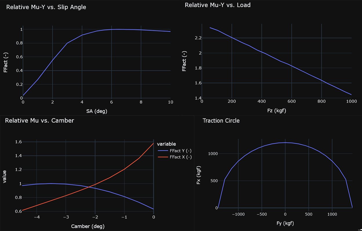
In this data grip was mostly given as a relative force metric “FFact”, probably so that the actual absolute force values could be obfuscated somewhat if this data is derived from a real source for these cars.
The slip angle curve has a fairly flat peak, where anything around between 6 and 7.5 degrees gives us most of the peak grip. There isn’t any info on the dependency of peak slip angle on things like camber, load, etc. In the sim data we can look for spikes beyond this region as signs of understeer/oversteer.
The load plot shows a strong dependence of Mu on load. One thing this will mean is that getting the balance of the car dialed in appropriately will be of extra importance. Weight transfer on a given axle will reduce it’s total grip proportionately, so the difference of how much weight transfer occurs between the front and rear will influence the balance between understeer/oversteer. On the vehicle setup end this can be controlled by spring rates and roll center heights.
For camber dependencies we were given trends for both FY and FX. For FY we see peak grip occuring around between -3 and -4 degrees. For FX we see a very dramatic trend where grip reduces by more than half going from 0 to -4 degrees. Pure longitudinal grip does tend to decrease with camber, but such a high sensitivity does not seem very realistic. One implication for this though would be that the FX potential of the tires would change rapidly through turn-entry and turn-exit as the camber change from body roll occurs. On turn-exit for example, the outside rear would lose longitudinal grip faster as the car unloads and negative camber increases, which could cause tightness.
For the traction circle plot we see a pretty broad, forgiving combined curve shape. Only the drive portion of the circle is given so we can assume that the braking is symmetric and there isn’t any need to worry about ply-steer effects.
Simulation
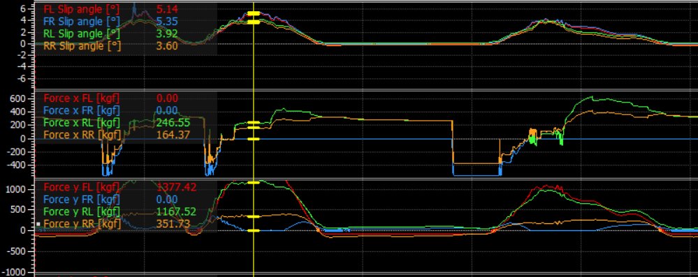
Lap simulation results were generated through the ChassisSim program, with a maximum limit of 100 runs to finalize the vehicle setup. Data was analyzed using Motec i2. Below for the baseline run through a left turn, we can see that the front right tire is lifting fully off the ground mid-corner (there is no FZ channel in the data but FY is clearly flatlining to 0). The fronts are also generating more slip angle with wheel, so both of these indicated the car needed to be freed up.
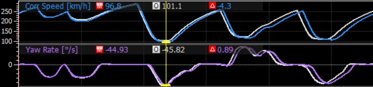
With lots of trial and error in the ChassisSim program adjusting spring rates, front view suspension geometry, static cambers, etc, a sizeable gain in speed was found. Below with the white trace for the final setup, significant time is being made up in this segment through some low speed turns.